Tutorial

Applying PSMC to simulated data

Published 2015-07-10

This is a simple tutorial showing how to use PSMC to infer the population-size history from full DNA sequences. We will apply PSMC to simulated data.

We need:

• The ms software.
• The PSMC software.
• Two Python scripts (one for converting files and the other for plotting the results).

Downloading and compiling software

Download and compile ms

Go to http://home.uchicago.edu/rhudson1/source/mksamples.html and download the file ms.tar.gz. Uncompress the file:

tar -zxvf ./ms.tar

Compile ms:

cd msdir
gcc -O3 -o ms ms.c streec.c rand1.c -lm

Have a look at the ms readme file for more details. The original paper can be viewed here.

Download and compile PSMC

Clone the GitHub repository:

git clone https://github.com/lh3/psmc.git

Compile:

cd psmc
make
cd utils
make

The PSMC model was published by Li and Durbin in 2011. For the analysis we will generate a dataset similar to the first dataset used in the supplementary materials of that paper.

Download the Python scripts

git clone https://github.com/willyrv/ms-PSMC.git

Finally, create a new folder and copy the binary files ./msdir/ms and ./psmc/psmc as well as the Python scripts.

Simulating data and running the analysis

I will suppose you have all these files in a folder:

|- ms
|- psmc
|- ms2psmcfa.py
|- plot_results.py

You need to verify that the files have execution permissions. To give execution permissions to the files:

chmod +x ./*

1. Simulate the data with ms

./ms 2 100 -t 30000 -r 6000 30000000 -eN 0.01 0.1 -eN 0.06 1 -eN  0.2 0.5 -eN 1 1 -eN 2 2 -p 8  > sim1.ms

This step is usually fast and should produce one output file (here called sim1.ms). Now we will use the ms2psmcfa.py Python script to convert this ms output into the input file of PSMC.

2. Convert the ms output

./ms2psmcfa.py ./sim1.ms > sim1.psmcfa

This creates the file sim1.psmcfa, which is the input of PSMC. Now we can run the PSMC analysis. For explanations of the parameters, see the README file of PSMC.

3. Run PSMC

./psmc -N25 -t15 -r5 -p 4+25*2+4+6 -o dem_history_sim1.psmc ./sim1.psmcfa

This can take a long time (about three hours in the original 2015 run). A copy of the original result file remains available: dem_history_sim1.psmc.

Once the PSMC analysis is finished, you can plot the results.

4. Plot the results

./plot_results.py

You should obtain a figure with the inferred demographic history (dashed blue line) and the real history (continuous black line) corresponding to the ms command.

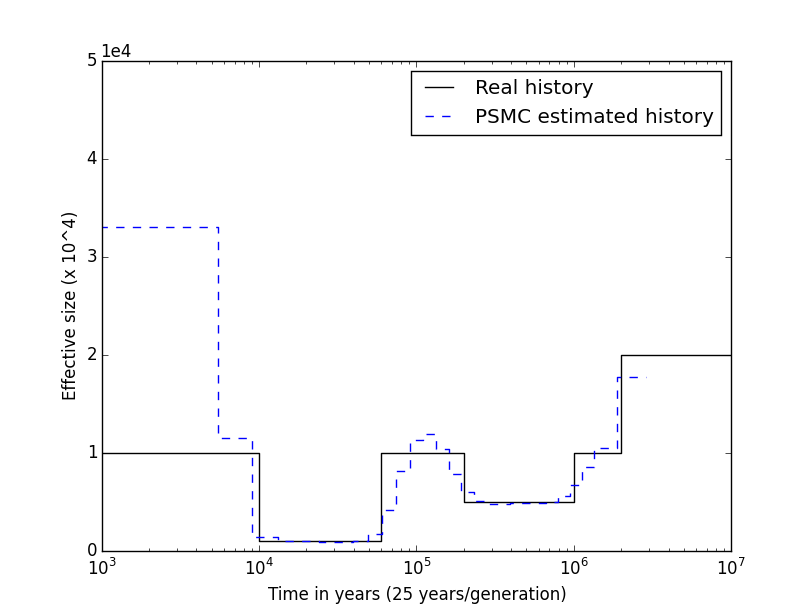
You can also plot the PSMC results by using the Perl script utils/psmc_plot.pl which comes with the PSMC software.

See also the later papers on the IICR for the interpretation of such curves under structured models.